Michal ZimmermannPieces of knowledge from the world of GIS.

Articles tagged with svg tag

Plotting the Czech Cadastre Land Use with d3: Data Viz (part IV)

This post is the fourth part of the series summarizing the process of visualizing land use data with bash, PostgreSQL and d3.js. Read other parts:

  1. Plotting the Czech Cadastre Land Use with d3: Data Extraction (part I)
  2. Plotting the Czech Cadastre Land Use with d3: Data Transformation (part II)
  3. Plotting the Czech Cadastre Land Use with d3: Data Load (part III)

Data vizualization

Those of you who’ve been following this series know all the data are set and ready to be used. The rest of you, shame on you by the way, can go through the above posts to catch up.

The result is available at https://www.zimmi.cz/kn-landuse-monitor and works like the gif below.

Features

Todos

Technologies

I implemented the whole app with vanilla JavaScript. The app resided in the Monitor variable, had several modules that were communicating via custom events with each other.

So far, so good. Once the app was production-ready, I stumbled upon vue.js, which is by miles the best JavaScript framework experience I’ve had so far. Reinventing the app once again was the matter of two days (thanks to this amazing setup - hot reload included).

Thus, the current version of the app is based on:

vue.js

Thanks to the easy-to-understand system of components, properties and methods, learning curve is really steep. The app is now divided into several components (Search, Dashboard with child components for charts and similar cadastres list).

vuex

Vuex, probably inspired by Flux or Redux, is the “state management pattern + library”, the single source of truth for your apps. That’s pretty much it: there’s only one place in your app (called the store), where you go to put or get your data. Not necessarily every single piece of data, just those pieces used across several components. It plays really nice with the vue.js.

D3.js

Tried it before, D3.js was really hard to grasp. And it still is, I guess. At the same time, it’s damn good at plotting the data. Yet, being a bit less low-level would be great.

Dexie

I hate writing servers for my pet projects. The server means no Github Pages. Thus, I decided to load the whole dataset with fetch API from the external JSON file. Loading the 13K objects × 30 properties × array with 8 items in each didn’t seem like the best idea ever, so… Here comes Dexie, a IndexedDB API wrapper that makes it easy on you (unlike the IndexedDB API itself, which doesn’t even let you find out whether the database you’re creating already exists. Seriously?).

Dexie loads the initial dataset into the IndexedDB storage and reads it every time user comes back without loading the JSON file again. On data change, the fresh file will be loaded, the database flushed and the new data written. Behold; I hate the way it’s written.

Flex

Used flex for the first time, I’m not sure I understand how it actually works though. CSS feels more complicated every time I need it.

Bottom line: I use localStorage to keep track of the database existence.

Resume

Two pet projects completed in one month definitely means the winter is here! Looking forward to using more vue.js.
Plotting the Czech Cadastre Land Use with d3: Data Load (part III)

This post is the third part of the series summarizing the process of visualizing landuse data with bash, PostgreSQL and d3.js. Read other parts:

  1. Plotting the Czech Cadastre Land Use with d3: Data Extraction (part I)
  2. Plotting the Czech Cadastre Land Use with d3: Data Transformation (part II)
  3. you’re reading it now

ETL process

Before the d3 viz can be crafted, it’s necessary to:

  1. extract CSV data from the URLs provided via the Atom feed
  2. transform those data into a relational database, do some math
  3. load data into a d3.js viz
  4. profit (as usual)

Extract

See Plotting the Czech Cadastre Land Use with d3: Data Extraction (part I).

Transform

See Plotting the Czech Cadastre Land Use with d3: Data Transformation (part II).

Load

Thanks to the way I transformed the data, the whole load is done with simple

#!/bin/bash

touch ./data/data.js
echo "let data =" > ./data/data.js

(
cat << EOF | psql -qAt --no-psqlrc
    SELECT
    array_to_json(array_agg(row_to_json(r)))
    FROM (
    SELECT *
    FROM data
    ) r
EOF
) >> ./data/data.js

That’s the whole ETL process! Next time, I’ll cover the d3.js viz.

Plotting the Czech Cadastre Land Use with d3: Data Transformation (part II)

This post is the second part of the series summarizing the process of visualizing landuse data with bash, PostgreSQL and d3.js. Read other parts:

  1. Plotting the Czech Cadastre Land Use with d3: Data Extraction (part I)
  2. you’re reading it now
  3. Plotting the Czech Cadastre Land Use with d3: Data Transformation (part III)

ETL process

Before the d3 viz can be crafted, it’s necessary to:

  1. extract CSV data from the URLs provided via the Atom feed
  2. transform those data into a relational database, do some math
  3. load data into a d3.js viz
  4. profit (as usual)

Extract

See Plotting the Czech Cadastre Land Use with d3: Data Extraction (part I).

Transform

Last time, I extracted the data from multiple CSV files to separate PostgreSQL tables named by data_YYYYMMDD pattern. My current goal is to transform it into the one big data table, where each row represents one cadastral area. Here’s what I’m trying to achieve:

-[ RECORD 1 ]----------+----------------------------------
ku_kod                 | 600881
ku_nazev               | Bantice
celkova_vymera         | {3763255,3763255,3763256,3763256}
celkovy_pocet_parcel   | {670,668,664,667}
chmelnice_pp           | {0,0,0,0}
chmelnice_pp_r         | {0.00,0.00,0.00,0.00}
chmelnice_v            | {0,0,0,0}
chmelnice_v_avg        | {0,0,0,0}
chmelnice_v_r          | {0.00,0.00,0.00,0.00}
lesni_pozemek_pp       | {25,25,25,25}
lesni_pozemek_pp_r     | {3.73,3.74,3.77,3.75}
lesni_pozemek_v        | {83879,83879,83879,83879}
lesni_pozemek_v_avg    | {3355,3355,3355,3355}
lesni_pozemek_v_r      | {2.23,2.23,2.23,2.23}
orna_puda_pp           | {88,88,89,89}
orna_puda_pp_r         | {13.13,13.17,13.40,13.34}
orna_puda_v            | {3066230,3066230,3066230,3066230}
orna_puda_v_avg        | {34844,34844,34452,34452}
orna_puda_v_r          | {81.48,81.48,81.48,81.48}
ostatni_plocha_pp      | {201,199,199,201}
ostatni_plocha_pp_r    | {30.00,29.79,29.97,30.13}
ostatni_plocha_v       | {283468,283468,283468,284562}
ostatni_plocha_v_avg   | {1410,1424,1424,1416}
ostatni_plocha_v_r     | {7.53,7.53,7.53,7.56}
ovocny_sad_pp          | {0,0,0,0}
ovocny_sad_pp_r        | {0.00,0.00,0.00,0.00}
ovocny_sad_v           | {0,0,0,0}
ovocny_sad_v_avg       | {0,0,0,0}
ovocny_sad_v_r         | {0.00,0.00,0.00,0.00}
ttp_pp                 | {44,44,44,45}
ttp_pp_r               | {6.57,6.59,6.63,6.75}
ttp_v                  | {49002,49002,49002,47908}
ttp_v_avg              | {1114,1114,1114,1065}
ttp_v_r                | {1.30,1.30,1.30,1.27}
vinice_pp              | {1,1,1,1}
vinice_pp_r            | {0.15,0.15,0.15,0.15}
vinice_v               | {106178,106178,106178,106178}
vinice_v_avg           | {106178,106178,106178,106178}
vinice_v_r             | {2.82,2.82,2.82,2.82}
vodni_plocha_pp        | {23,23,23,23}
vodni_plocha_pp_r      | {3.43,3.44,3.46,3.45}
vodni_plocha_v         | {27877,27877,27877,27877}
vodni_plocha_v_avg     | {1212,1212,1212,1212}
vodni_plocha_v_r       | {0.74,0.74,0.74,0.74}
zahrada_pp             | {115,115,115,115}
zahrada_pp_r           | {17.16,17.22,17.32,17.24}
zahrada_v              | {77381,77381,77353,77353}
zahrada_v_avg          | {673,673,673,673}
zahrada_v_r            | {2.06,2.06,2.06,2.06}
zastavena_plocha_pp    | {173,173,168,168}
zastavena_plocha_pp_r  | {25.82,25.90,25.30,25.19}
zastavena_plocha_v     | {69240,69240,69269,69269}
zastavena_plocha_v_avg | {400,400,412,412}
zastavena_plocha_v_r   | {1.84,1.84,1.84,1.84}

Several stats were calculated for each land use category (vinice → vineyard, ovocny_sad → orchard, …):

All statistical columns are kept as PostgreSQL ARRAYs, ordered by dates (very handy for the future d3.js viz by the way).

Note that since the FULL OUTER JOIN is needed in the next step, SQLite can’t be used. Pity though.

The whole transformation bash script is the plain:

#!/bin/bash

psql -qAt --no-psqlrc -f transform.sql | psql -qAt --no-psqlrc

The transform.sql file is used to build the dynamic SQL query, which - once built - is piped to another psql command. I admit, pipes are super awesome.

WITH tables AS (
-- FULL OUTER JOIN all the data_YYYYMMDD tables
SELECT
    table_name,
    table_schema,
    'd' || id tbl,
    CASE WHEN id = 1
        THEN table_schema || '.' || table_name || ' d' || id
        ELSE 'FULL OUTER JOIN ' || table_schema || '.' || table_name || ' d' || id || ' ON (d1.ku_kod = d' || id || '.ku_kod)'
    END tbl_join
FROM (
    SELECT
        table_name,
        table_schema,
        row_number() OVER (ORDER BY table_name) id
    FROM information_schema.tables
    WHERE table_name LIKE 'data_%'
        AND table_type = 'BASE TABLE'
        AND table_schema = 'public'
) a
)
-- create data table with the correct values order for each statistical column
-- note that the whole process would crash if d1.ku_kod would be NULL -> @todo fix me
SELECT 'DROP TABLE IF EXISTS data;
    CREATE TABLE data AS
    SELECT d1.ku_kod, d1.ku_nazev,'
UNION ALL
SELECT
    array_to_string(array_agg(r), ', ') r
FROM (
    SELECT
    'ARRAY[' || array_to_string(array_agg(tables.tbl || '.' || columns.column_name ORDER BY tables.table_name), ', ') || ']' || ' ' || columns.column_name r
    FROM tables
    JOIN (
    SELECT
        table_schema,
        table_name,
        column_name
    FROM information_schema.columns
    WHERE column_name NOT LIKE 'ku_%'
    ORDER BY ordinal_position
    ) columns
    ON (tables.table_name = columns.table_name AND columns.table_schema = tables.table_schema)
    GROUP BY columns.column_name
) a
UNION ALL
SELECT 'FROM'
UNION ALL
SELECT tbl_join FROM tables;

psql -qAt --no-psqlrc -f transform.sql builds the actual query from the query above, | psql -qAt --no-psqlrc sends it to the database again. This part was really fun to implement!

I’m still considering to store diff values instead of absolute values in those ARRAYs - that would save some serious bandwidth!

Load

See Plotting the Czech Cadastre Land Use with d3: Data Transformation (part III).

Plotting the Czech Cadastre Land Use with d3: Data Extraction (part I)

This post is the first part of the upcoming series summarizing the process of visualizing landuse data with bash, PostgreSQL and d3.js. Read other parts:

  1. you’re reading it now
  2. Plotting the Czech Cadastre Land Use with d3: Data Transformation (part II)
  3. Plotting the Czech Cadastre Land Use with d3: Data Transformation (part III)

Czech Office for Surveying, Mapping and Cadastre has recently published lot of data via Atom feed. There’s pretty small and a bit boring dataset included, featuring quarterly updated landuse-related values for all 13,091 cadastral areas:

Data are published as CSV files linked from the Atom feed. Sadly, they come windows-1250 encoded, using Windows line endings, with trailing semicolons and header rows using diacritics.

ETL process

Before the d3 viz can be crafted, it’s necessary to:

  1. extract CSV data from the URLs provided via the Atom feed
  2. transform those data into a relational database, do some math
  3. load data into a d3.js viz
  4. profit (as usual)

Extract

#!/bin/bash
# extract.sh -f YYYYMMDD

while [[ $# -gt 1 ]]
do
key="$1"

case $key in
    -f|--file)
    FILE="$2"
    shift # past argument
    ;;
    *)
        # unknown option
    ;;
esac
shift # past argument or value
done

URL=http://services.cuzk.cz/sestavy/UHDP/UHDP-
CSVFILE=$FILE.csv
CSVUTF8FILE=${CSVFILE%.*}.utf.csv
URL+=$CSVFILE

echo "downloading $URL"
wget -q $URL -O $CSVFILE

if [[ $? != 0 ]]; then
    rm -f $CSVFILE
    echo "download failed"
    exit
fi

echo "converting to utf-8"
iconv -f WINDOWS-1250 -t UTF-8 $CSVFILE -o $CSVUTF8FILE && \
echo "modifying ${FILE}"
sed -i 's/^M$//' $CSVUTF8FILE && \
sed -i 's/\r$//' $CSVUTF8FILE && \
sed -i 's/;*$//g' $CSVUTF8FILE && \
sed -i '1d' $CSVUTF8FILE

echo "importing to database"
sed -e "s/\${DATE}/$FILE/g" extract.sql | psql -qAt --no-psqlrc

rm $CSVFILE $CSVUTF8FILE

This script downloads CSV file, deals with all the pitfalls mentioned above and, when done, copy command within extract.sql loads the data into a data_YYYYMMDD table. Putting all the files into the one table would have saved me a lot of transformation SQL, yet it didn’t feel quite right though.

Transform

See Plotting the Czech Cadastre Land Use with d3: Data Transformation (part II).

Load

See Plotting the Czech Cadastre Land Use with d3: Data Transformation (part III).

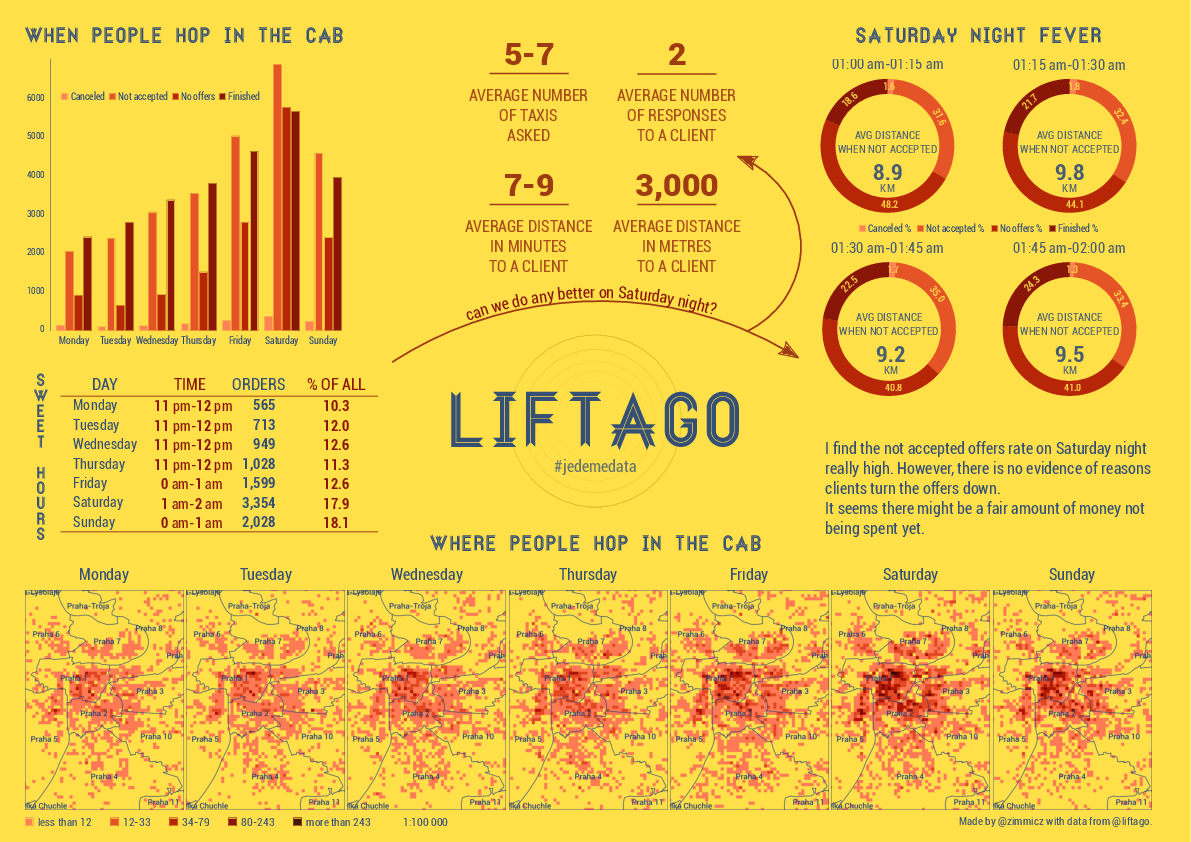
Liftago Open Dataset Infographics

Liftago (the Czech analogy of Uber) has recently released a sample of its data covering four weeks of driver/pasenger interactions.

Have a look at my infographics created with PostGIS, Inkscape, Python and pygal.