Liftago Open Dataset Infographics
Liftago (the Czech analogy of Uber) has recently released a sample of its data covering four weeks of driver/pasenger interactions.
Have a look at my infographics created with PostGIS, Inkscape, Python and pygal.
Liftago (the Czech analogy of Uber) has recently released a sample of its data covering four weeks of driver/pasenger interactions.
Have a look at my infographics created with PostGIS, Inkscape, Python and pygal.
After a while I got back to my PostGIS open data case study. Last time I left it with clustering implemented, looking forward to incorporate Turf.js in the future. And the future is now. The code is still available on GitHub.
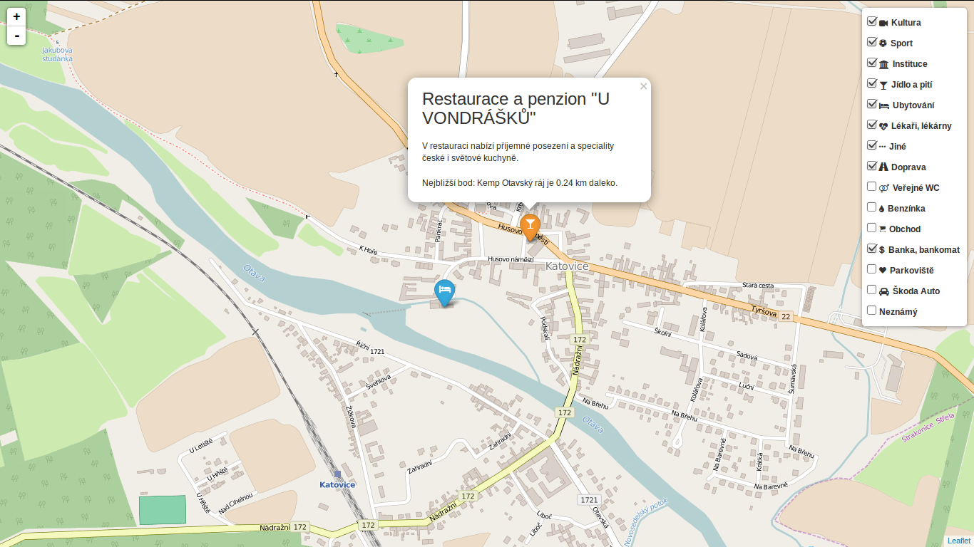
Vozejkmap data is categorized based on the place type (banks, parking lots, pubs, …). One of the core features of map showing such data should be the easy way to turn these categories on and off.
As far as I know, it’s not trivial to do this with the standard Leaflet library. Extending L.control.layers and implement its addOverlay, removeOverlay methods on your own might be the way to add needed behavior. Fortunately, there’s an easier option thanks to Leaflet.FeatureGroup.SubGroup that can handle such use case and is really straightforward. See the code below.
cluster = L.markerClusterGroup({
    chunkedLoading: true,
    chunkInterval: 500
});

cluster.addTo(map);

...

for (var category in categories) {
    // just use L.featureGroup.subGroup instead of L.layerGroup or L.featureGroup
    overlays[my.Style.set(category).type] = L.featureGroup.subGroup(cluster, categories[category]);
}

mapkey = L.control.layers(null, overlays).addTo(map);
With this piece of code you get a map key with checkboxes for all the categories, yet they’re still kept in the single cluster on the map. Brilliant!

Turf is one of those libraries I get amazed easily with, spending a week trying to find a use case, finally putting it aside with “I’ll get back to it later”. I usually don’t. This time it’s different.
I use Turf to get the nearest neighbor for any marker on click. My first try ended up with the same marker being the result as it was a member of a feature collection passed to turf.nearest() method. After snooping around the docs I found turf.remove() method that can filter GeoJSON based on key-value pair.
Another handy function is turf.distance() that gives you distance between two points. The code below adds an information about the nearest point and its distance into the popup.
// data is a geojson feature collection
json = L.geoJson(data, {
    onEachFeature: function(feature, layer) {
        layer.on("click", function(e) {
            var nearest = turf.nearest(layer.toGeoJSON(), turf.remove(data, "title", feature.properties.title)),
                distance = turf.distance(layer.toGeoJSON(), nearest, "kilometers").toPrecision(2),
                popup = L.popup({offset: [0, -35]}).setLatLng(e.latlng),
                content = L.Util.template(
                    "<h1>{title}</h1><p>{description}</p> \
                    <p>Nejbližší bod: {nearest} je {distance} km daleko.</p>", {
                    title: feature.properties.title,
                    description: feature.properties.description,
                    nearest: nearest.properties.title,
                    distance: distance
                });

            popup.setContent(content);
            popup.openOn(map);

            ...
From what I’ve tried so far, Turf seems to be incredibly fast and easy to use. I’ll try to find the nearest point for any of the categories, that could take Turf some time.
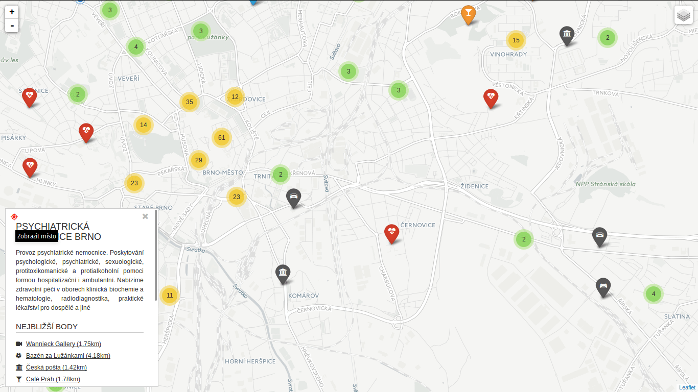
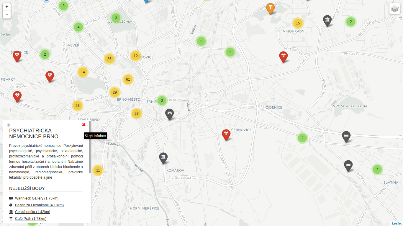
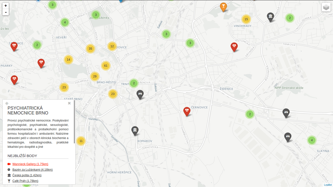
Turf is blazing fast! I’ve implemented nearest point for each of the categories and it gets done in a blink of an eye. Some screenshots below. Geolocation implemented as well.
 You can locate the point easily.
 You can hide the infobox.
 You can jump to any of the nearest places.
I’ve seen a bunch of questions on GIS StackExchange recently related to SFCGAL extension for PostGIS 2.2. Great news are it can be installed with one simple query CREATE EXTENSION postgis_sfcgal. Not so great news are you have to compile it from source for Ubuntu-based OS (14.04) as recent versions of required packages are not available in the repositories.
I tested my solution on elementary OS 0.3.1 based on Ubuntu 14.04. And it works! It installs PostgreSQL 9.4 from repositories together with GDAL and GEOS and some other libs PostGIS depends on. PostGIS itself, CGAL, Boost, MPFR and GMP are built from source.
Here comes the code (commented where needed).
sudo -i
echo "deb http://apt.postgresql.org/pub/repos/apt/ trusty-pgdg main" | tee -a /etc/apt/sources.list
wget --quiet -O - https://www.postgresql.org/media/keys/ACCC4CF8.asc | sudo apt-key add -
apt-get update
apt-get install -y postgresql-9.4 \
    postgresql-client-9.4 \
    postgresql-contrib-9.4 \
    libpq-dev \
    postgresql-server-dev-9.4 \
    build-essential \
    libgeos-c1 \
    libgdal-dev \
    libproj-dev \
    libjson0-dev \
    libxml2-dev \
    libxml2-utils \
    xsltproc \
    docbook-xsl \
    docbook-mathml \
    cmake \
    gcc \
    m4 \
    icu-devtools

exit # leave root otherwise postgis will choke

cd /tmp
touch download.txt
cat <<EOT >> download.txt
https://gmplib.org/download/gmp/gmp-6.0.0a.tar.bz2
https://github.com/Oslandia/SFCGAL/archive/v1.2.0.tar.gz
http://www.mpfr.org/mpfr-current/mpfr-3.1.3.tar.gz
http://downloads.sourceforge.net/project/boost/boost/1.59.0/boost_1_59_0.tar.gz
https://github.com/CGAL/cgal/archive/releases/CGAL-4.6.3.tar.gz
http://download.osgeo.org/postgis/source/postgis-2.2.0.tar.gz

EOT

cat download.txt | xargs -n 1 -P 8 wget # make wget a little bit faster

tar xjf gmp-6.0.0a.tar.bz2
tar xzf mpfr-3.1.3.tar.gz
tar xzf v1.2.0.tar.gz
tar xzf boost_1_59_0.tar.gz
tar xzf CGAL-4.6.3.tar.gz
tar xzf postgis-2.2.0.tar.gz

CORES=$(nproc)

if [[ $CORES > 1 ]]; then
    CORES=$(expr $CORES - 1) # be nice to your PC
fi

cd gmp-6.0.0
./configure && make -j $CORES && sudo make -j $CORES install

cd ..
cd mpfr-3.1.3
./configure && make -j $CORES && sudo make -j $CORES install

cd ..
cd boost_1_59_0
./bootstrap.sh --prefix=/usr/local --with-libraries=all && sudo ./b2 install # there might be some warnings along the way, don't panic
echo "/usr/local/lib" | sudo tee /etc/ld.so.conf.d/boost.conf
sudo ldconfig

cd ..
cd cgal-releases-CGAL-4.6.3
cmake . && make -j $CORES && sudo make -j $CORES install

cd ..
cd SFCGAL-1.2.0/
cmake . && make -j $CORES && sudo make -j $CORES install

cd ..
cd postgis-2.2.0
./configure \
    --with-geosconfig=/usr/bin/geos-config \
    --with-xml2config=/usr/bin/xml2-config \
    --with-projdir=/usr/share/proj \
    --with-libiconv=/usr/bin \
    --with-jsondir=/usr/include/json \
    --with-gdalconfig=/usr/bin/gdal-config \
    --with-raster \
    --with-topology \
    --with-sfcgal=/usr/local/bin/sfcgal-config && \
make && make cheatsheets && sudo make install # deliberately one CPU only

sudo -u postgres psql
sudo -u postgres createdb spatial_template
sudo -u postgres psql -d spatial_template -c "CREATE EXTENSION postgis;"
sudo -u postgres psql -d spatial_template -c "CREATE EXTENSION postgis_topology;"
sudo -u postgres psql -d spatial_template -c "CREATE EXTENSION postgis_sfcgal;"
sudo -u postgres psql -d spatial_template -c "SELECT postgis_full_version();"
As mentioned in QGIS Tips For Collaborative Mapping we’re in the middle of crop evaluation project at CleverMaps.
With the QGIS workflow up and running, I’ve been focused on different QGIS related task: automatic map generation for land blocks that meet certain conditions. The logic behind identifying such land blocks is as follows:
Let’s assume that with several lines of SQL code we can store these mentioned above in a table called land_blocks with geometries being the result of calling ST_Union() over parcels for each land block.
Every map should feature following layers:
land_blocks table?) - labeled with ID, yellowish borders, no fillLabels should be visible only for the featured land block (both for the land parcels and the land block itself. The whole map scales dynamically, showing small land blocks zoomed in and the large ones zoomed out.
Every map features additional items:
Now with requirements defined, let’s create some maps. It’s incredibly easy to generate a series of maps with QGIS atlas options.
Coverage layer is presumably the only thing you really need - as the name suggests, it covers your area of interest. One map will be created for each feature in this layer, unless you decide to use some filtering - which I did.
Output filenames can be tweaked to your needs, here’s what such a function might look like. If there is a slash in the land block ID (XXXXXXX/Y), the filename is set to USER-ID_XXXXXXX-00Y_M_00, USER-ID_XXXXXXX-000_M_00 otherwise.
CASE WHEN strpos(attribute($atlasfeature, 'kod_pb'), '/') > -1
    THEN
        ji || '_' ||
        substr(
            attribute($atlasfeature, 'kod_pb'), 0,
            strpos(attribute($atlasfeature, 'kod_pb'), '/')+1 -- slash position
        ) || '-' ||
        lpad(
            substr(
                attribute($atlasfeature, 'kod_pb'),
                strpos(attribute($atlasfeature, 'kod_pb'), '/') + 2,
                length(attribute($atlasfeature, 'kod_pb'))
            ),
        3, '0') || '_M_00'
    ELSE
        ji || '_' || attribute($atlasfeature, 'kod_pb') || '-000_M_00'
END
Different land blocks are of different sizes, thus needing different scales to fit in the map. Again, QGIS handles this might-become-a-nightmare-pretty-easily issue with a single click. You can define the scale as:
With these settings, I get a map similar to the one below. Notice two interesting things:
[something in the brackets] notations. These will be substituted with actual values during the atlas generation. Showing land block ID with a preceeding label is as easy as [%concat('PB: ', "kod_pb")%] (mind the percentage sign).Atlas features are a great help for map customization. As mentioned earlier, in my case, only one land block label per map should be visible. That can be achieved with a simple label dialog expression:
CASE
    WHEN $id = $atlasfeatureid
    THEN "kod_pb"
END
QGIS keeps reference to each coverage layer feature ID during atlas generation, so you can use it for comparison. The best part is you can use IDs with any layer you need:
CASE
    WHEN attribute($atlasfeature, 'kod_pb') = "kod_pb"
    THEN "kod_zp"
END
With this simple expression, I get labels only for those land parcels that are part of the mapped land block. Even the layer style can be controlled with atlas feature. Land parcels inside the land block have blue borders, the rest is yellowish, remember? It’s a piece of cake with rule-based styling.
When you’re set, atlas can be created with a single button. I used SVG as an output format to easily manipulate the map content afterwards. The resulting maps look like the one in the first picture without the text in the red rectangle. A Python script appends this to each map afterwards.
Roughly speaking, generating 300 maps takes an hour or so, I guess that depends on the map complexity and hardware though.
SVG output is just plain old XML that you can edit by hand or by script. A simple Python script, part of map post-processing, loads SVG from the database and adds it to the left pane of each map.
SELECT
      ji,
      kod_pb,
      concat(
            '<g fill="none" stroke="#000000" stroke-opacity="1" stroke-width="1"
                  stroke-linecap="square" stroke-linejoin="bevel" transform="matrix(1.18081,0,0,1.18081,270.0,550.0)"
                  font-family="Droid Sans" font-size="35" font-style="normal">',
            kultura, vymery, vymery_hodnoty,
            vcs_titul, vcs_brk, vcs_brs, vcs_chmel,
            vcs_zvv, vcs_zv, vcs_ovv, vcs_ov, vcs_cur, vcs_bip,
            lfa, lfa_h1, lfa_h2, lfa_h3,
            lfa_h4, lfa_h5, lfa_oa, lfa_ob, lfa_s,
            natura, aeo_eafrd_text, dv_aeo_eafrd_a1,
            dv_aeo_eafrd_a2o, dv_aeo_eafrd_a2v, dv_aeo_eafrd_b1,
            dv_aeo_eafrd_b2, dv_aeo_eafrd_b3, dv_aeo_eafrd_b4,
            dv_aeo_eafrd_b5, dv_aeo_eafrd_b6, dv_aeo_eafrd_b7,
            dv_aeo_eafrd_b8, dv_aeo_eafrd_b9, dv_aeo_eafrd_c1,
            dv_aeo_eafrd_c3, aeko_text, dv_aeko_a, dv_aeko_b, dv_aeko_c,
            dv_aeko_d1, dv_aeko_d2, dv_aeko_d3, dv_aeko_d4, dv_aeko_d5,
            dv_aeko_d6, dv_aeko_d7, dv_aeko_d8, dv_aeko_d9, dv_aeko_d10,
            dv_aeko_e, dv_aeko_f, ez, dzes_text, rep, obi, seop, meop, pbz, dzes7,
            '</g>'
      ) popis
FROM (...);
Each column from the previous query is a result of SELECT similar to the one below.
SELECT concat('<text fill="#000000" fill-opacity="1" stroke="none">BrK: ', dv_brk, ' ha / ', "MV_BRK", ' ha;', kod_dpz, '</text>') vcs_brk
The transform="matrix(1.18081,0,0,1.18081,270.0,550.0) part puts the text on the right spot. Great finding about SVG is that it places each <text> element on the new line, so you don’t need to deal with calculating the position in your script.
Scale adjustment is done with a dirty lambda function.
content = re.sub(r">(\d{1,3}\.\d{3,5})</text>", lambda m :"> " + str(int(round(float(m.group(1))))) + "</text>", old_map.read())
We deliver maps as JPEG files with 150 DPI on A4 paper format. ImageMagick converts the formats with a simple shell command:
convert -density 150 -resize 1753x1240 input.svg output.jpg
I created pretty efficient semi-automated workflow using several open source technologies that saves me a lot of work. Although QGIS has some minor pet peeves (scale with decimal places, not showing the entire feature, not substituting variables at times), it definitely makes boring map creation quite amusing. The more I work with big data / on big tasks, the more I find Linux a must-have.
The whole process was done with QGIS 2.10, PostGIS 2.1, PostgreSQL 9.3, Python 2.7, ImageMagick 6.7.
Filtering really big (millions of rows) point datasets by distance might get catchy when solved with wrong PostGIS functions. Without spatial indexes PostGIS would take ages to finish such task.
Someone over StackExchange asked why the next query had been running for 15 hours (!) with no result:
SELECT
    a.gid,
    b.gid,
    ST_Distance(a.geom,b.geom)
FROM
    shp1 a,
    shp2 b
WHERE
    ST_Intersects(
        ST_Difference(
            ST_Buffer(a.geom,2000),
            ST_Buffer(a.geom,500)
        ),
        b.geom
    ) AND
    abs(a.value - b.value) > 400
The answer is quite simple: because it was using wrong functions. Let’s see:
ST_Distance() does not use spatial index, it’s a simple mathematical calculation, it’s expensive and it can be replaced by spatial operator for point datasets.ST_Buffer() will definitely take time to build polygons around points. And it’s being run twice!ST_Difference() needs more time to compare the buffers and return just the portion of space they don’t share. Isn’t it a huge waste to create buffers and then throw them away?ST_Intersects() finally checks whether the point should be included in the result.That was a great challenge to test my knowledge of how PostGIS works and here’s my shot at it:
SELECT * FROM (
    SELECT
        a.gid,
        b.gid,
        a.geom <-> b.geom distance
    FROM
        shp1 a, shp2 b
    WHERE
        abs(a.value - b.value) > 400 AND
        ST_DWithin(a.geom, b.geom, 2000)
    ) sq
WHERE
    distance > 500;
<->, a.k.a geometry distance centroid instead of ST_Distance(). It takes advantage of spatial indexes, thus it’s fast. And it’s perfectly fine to use it with point dataset, because the centroid of a bounding box of a point is? That point, exactly. Spatial indexes have to be built beforehand.ST_Dwithin() was made for. With the inner WHERE clause I get all the points lying at most 2,000 meters from the current, having the absolute value difference bigger than 400. ST_Dwithin() will make use of any spatial index available, unlike ST_Distance().WHERE clause throws away all the points closer than 500 meters. Remember, we already got only those not further than 2,000 meters from the previous step.It took PostGIS 1060545,590 ms (~ 17 minutes) on my Quad-Core Intel® Core™ i5-4210M CPU @ 2.60GHz, 4 GB RAM, 500 GB SSD hard drive, PostgreSQL 9.3 and PostGIS 2.1 with two point datasets having 4M and 300K rows, respectively.