Articles tagged with gdal tag
As I’m still running Ubuntu 16.04 based Linux Mint, I have no access to GDAL 2.x repositories (except for ubuntugis, that I really don’t like to use). Provided with a GeoPackage raster file recently, I had to find a way to load it into QGIS, somehow. The solution is simple: Docker with gdal_translate.
Preparing the Docker container
I like using Docker for experiments that might leave the OS in an unexpected state (which is exactly what happens to me with ubuntugis repository whenever I use it. That’s why I don’t anymore.). A very simple Dockerfile keeps the troubles away from you.
FROM ubuntu:17.04
RUN apt update
RUN apt install -y gdal-bin
cd into the folder and build the image with docker build -t gdal .. Once ready, summon the daemon, run the container, mount the GeoPackage file to the container directory and you’re ready to rock.
docker run -v /path/to/geopackage:/home/ -it gdal
Raster GeoPackage to GeoTiff translation
With the container running, the raster GeoPackage to GeoTiff translation can be done easily with gdal_translate. Note I chose to cut the source file into tiles, because the gdal_translate was choking about the resulting size.
#!/bin/bash
SIZE=10000
ULX=-630000
ULY=-1135450
LRX=-560000
LRY=-1172479
COUNTER_X=0
COUNTER_Y=0

while [[ $ULX -lt $LRX ]]
do
    while [[ $ULY -gt $LRY ]]
    do
        echo $ULX, $(($ULX+$SIZE)), $ULY, $(($ULY-$SIZE))

        gdal_translate \
            -co TILED=YES \
            -co COMPRESS=DEFLATE \
            -co TFW=YES \
            -co NUM_THREADS=ALL_CPUS \
            -a_nodata 0 \
            -of GTiff \
            -projwin $ULX, $ULY, $(($ULX+$SIZE)), $(($ULY-$SIZE)) \
            -projwin_srs EPSG:5514 \
            data/detected.gpkg data/detected_${COUNTER_X}_${COUNTER_Y}.tiff

        ULY=$(($ULY-$SIZE))
        COUNTER_Y=$((COUNTER_Y+1))
    done
    ULX=$(($ULX+$SIZE))
    ULY=-1135450
    COUNTER_X=$((COUNTER_X+1))
done
Final Touch: Raster to Vector
After the GeoTiff is written to hard drive, inotifywait can be used to generate overviews. And with ease of calling gdal_polygonize.py on each of GeoTiffs…vector layer, at you service.
Today my workmate asked if there was a way to see an attribute table other than importing spatial data into a PostGIS database. I told him about QGIS and while talking about other GIS stuff, I started thinking about pipes and how awesome it would be to actually format the output of the ogrinfo command.
Here it is. It is just a much longer way to do ogr2ogr -f "CSV" dest source, but sometimes you just have to experiment a bit.
#!/bin/bash
FILE=$1

function columns {
    ogrinfo $FILE -al -so | \
    sed '/Column/,$!d' | \
    sed '/Geometry Column/d' | \
    sed -e 's/Column =/\:/g' | \
    awk -F: '{print $1}' | \
    awk -v RS= -v OFS="|" '{$1 = $1} 1'
}

function data {
   ogrinfo $FILE -al | \
   sed '/OGRFeature/,$!d' | \
   sed '/POLYGON\|LINESTRING\|POINT/ d' | \
   sed -e 's/OGRFeature\(.*\)\://g' | \
   sed -e 's/.*\s*\(.*\)\s*=\s*//g' | \
   awk -v RS= -v OFS="|" '{$1 = $1} 1'
}

{ columns; data; }
The result can be piped to other bash functions, such as less or more. I call it ogrinfotable.
PostgreSQL foreign data wrappers are used to connect PostgreSQL database to different datasources, e.g. other SQL databases, CSV files, XLS spreadsheets×
The one I’ve been interested in for several months is Paul Ramsey’s OGR FDW - it gives you access to OGR supported spatial formats directly from your database. No more shapefiles lying around?
Each foreign data wrapper should have three basic components:
- foreign server object
- foreign user mapping - not necessary if you’re not connecting to other database
- foreign table(s)
I got some data about rivers and dams from DIBAVOD open datasets to play with.
First define the foreign server object:
CREATE SERVER dibavod
FOREIGN DATA WRAPPER ogr_fdw
OPTIONS (
    datasource '/downloads/dibavod',
    format 'ESRI Shapefile',
    config_options 'SHAPE_ENCODING=CP1250'
);
Note the OGR specific driver configuration options are available inside config_options. In case of ESRI Shapefiles, the datasource is the directory your files reside in.
Let’s create PostgreSQL tables (use ogrinfo or Paul’s ogr_fdw_info to list the columns):
CREATE FOREIGN TABLE rivers (
    fid integer,
    utokj_id numeric,
    utokjn_id numeric,
    utokjn_f numeric,
    prprop_z integer,
    ex_jh integer,
    pozn text,
    shape_leng numeric,
    naz_tok text,
    idvt integer,
    tok_id numeric,
    shape_len numeric,
    geom geometry(LINESTRING, 5514)
)
SERVER dibavod
OPTIONS (layer 'A02_Vodni_tok_JU');

CREATE FOREIGN TABLE dams (
    fid integer,
    objectid integer,
    naz_na text,
    nadr_gid numeric,
    kota_hladi numeric,
    hloubka numeric,
    zatop_ploc numeric,
    objem numeric,
    kota_hraz numeric,
    kota_preli numeric,
    kota_vypus numeric,
    plocha_m2 numeric,
    shape_area numeric,
    shape_len numeric,
    geom geometry(MULTIPOLYGON, 5514)
)
SERVER dibavod
OPTIONS (LAYER 'A05_Vodni_nadrze');
Note the fid column - required for write access to underlying datasource.
Things to remember:
- foreign tables mean no constraints nor indices
- no indices mean spatial queries are terribly slow compared to PostGIS
- I like the idea of
CREATE UNLOGGED TABLE dams2 AS SELECT * FROM dams, not sure what to use it for though
We have to deal with DGN drawings quite often at CleverMaps - heavily used for infrastructure projects (highways, roads, pipelines), they are a pure nightmare to the GIS person inside me. Right now, I’m only capable of converting it into a raster file and serve it with Geoserver. The transformation from DGN to PDF to PNG to Tiff is not something that makes me utterly happy though.
All you need to do the same is GDAL, ImageMagick, some PDF documents created out of DGN files - something MicroStation can help you with - and their upper left and lower right corner coordinates.
# I recommend putting some limits on ImageMagick - it tends to eat up all the resources and quit
export MAGICK_MEMORY_LIMIT=1512
export MAGICK_MAP_LIMIT=512
export MAGICK_AREA_LIMIT=1024
export MAGICK_FILES_LIMIT=512
export MAGICK_TMPDIR=/partition/large/enough

# I expect two files on the input: the first is PDF file with drawing, the second is a simple text file with four coordinates on a single line in the following order: upper left x, upper left y, lower right x, lower right y
INPUT=${1:?"PDF file path"}
COORDS=${2:?"Bounding box file path"}
OUTPUTDIRNAME=$(dirname $INPUT)
OUTPUTFILENAME=$(basename $INPUT | cut -d. -f1).png
OUTPUTPATH=$OUTPUTDIRNAME/$OUTPUTFILENAME

# create PNG image - I actually don't remember why it didn't work directly to Tiff
gdal_translate \
    -co WORLDFILE=YES \
    -co ZLEVEL=5 \
    -of PNG \
    --config GDAL_CACHEMAX 500 \
    --config GDAL_PDF_DPI 300 \
    -a_srs EPSG:5514 \ # Czech local CRS
    -a_ullr $(echo $(cat $COORDS)) \ # read the file with coordinates
    $INPUT \
    $OUTPUTPATH

# convert to Tiff image
convert \
    -define tiff:tile-geometry=256x256 \
    -transparent white \ # drawings come with white background
    $OUTPUTPATH \
    ${OUTPUTPATH/.png}_alpha.tif

# build overwies to speed things up
gdaladdo ${OUTPUTPATH/.png}_alpha.tif 2 4 8 16 32
And you’re done. The .wld file will be present for each resulting file. I rename it manually to match the name of a GeoTiff - that should be probably done automatically as well.
The Digital Elevation Model over Europe (EU-DEM) has been recently released for public usage at Copernicus Land Monitoring Services homepage. Strictly speaking, it is a digital surface model coming from weighted average of SRTM and ASTER GDEM with geographic accuracy of 25 m. Data are provided as GeoTIFF files projected in 1 degree by 1 degree tiles (projected to EPSG:3035), so they correspond to the SRTM naming convention.
If you can’t see the map to choose the data to download, make sure you’re not using HTTPS Everywhere or similar browser plugin.
I chose Austria to play with the data.
Obtaining the data
It’s so easy I doubt it’s even worth a word. Get zipped data with wget, extract them to a directory.
wget https://cws-download.eea.europa.eu/in-situ/eudem/eu-dem/EUD_CP-DEMS_4500025000-AA.rar -O dem.rar
unrar dem.rar -d copernicus
cd copernicus
Hillshade and color relief
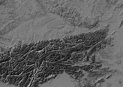
Use GDAL to create hillshade with a simple command. No need to use -s flag to convert units, it already comes in meters. Exaggerate heights a bit with -z flag.
gdaldem hillshade EUD_CP-DEMS_4500025000-AA.tif hillshade.tif -z 3
And here comes the Alps.

To create a color relief you need a ramp of heights with colors. “The Development and Rationale of Cross-blended Hypsometric Tints” by T. Patterson and B. Jenny is a great read on hypsometric tints. They also give advice on what colors to choose in different environments (see the table at the last page of the article). I settled for warm humid color values.
| Elevation [m] |
Red |
Green |
Blue |
| 5000 |
220 |
220 |
220 |
| 4000 |
212 |
207 |
204 |
| 3000 |
212 |
193 |
179 |
| 2000 |
212 |
184 |
163 |
| 1000 |
212 |
201 |
180 |
| 600 |
169 |
192 |
166 |
| 200 |
134 |
184 |
159 |
| 50 |
120 |
172 |
149 |
| 0 |
114 |
164 |
141 |
I created a color relief with another GDAL command.
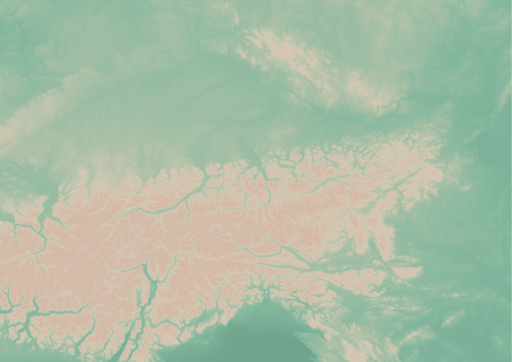
gdaldem color-relief EUD_CP-DEMS_4500025000-AA.tif ramp_humid.txt color_relief.tif
And here comes hypsometric tints.

Add a bit of compression and some overviews to make it smaller and load faster.
gdal_translate -of GTiff -co TILED=YES -co COMPRESS=DEFLATE color_relief.tif color_relief.compress.tif
gdal_translate -of GTiff -co TILED=YES -co COMPRESS=DEFLATE hillshade.tif hillshade.compress.tif
rm color_relief.tif
rm hillshade.tif
mv color_relief.compress.tif color_relief.tif
mv hillshade.compress.tif hillshade.tif
gdaladdo color_relief.tif 2 4 8 16
gdaladdo hillshade.tif 2 4 8 16
Map composition
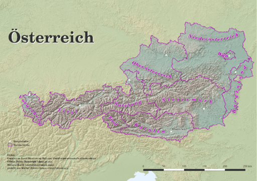
I chose Austria for its excessive amount of freely available datasets. What I didn’t take into consideration was my lack of knowledge when it comes to German (#fail). States come from data.gv.at and was dissolved from smaller administrative units. State capitals were downloaded from naturalearth.com.

I’d like to add some more thematic layers in the future. And translate the map to English.
Few words on INSPIRE Geoportal
INSPIRE Geoportal should be the first place you go to search for European spatial data (at last EU thinks so). I used it to find data for this map and it was a very frustrating experience. It was actually more frustrating than using Austrian open data portal in German. Last news are from May 21, 2015, but the whole site looks and feels like deep 90s or early 2000 at least.
