Ogrinfo Output Formatting

Today my workmate asked if there was a way to see an attribute table other than importing spatial data into a PostGIS database. I told him about QGIS and while talking about other GIS stuff, I started thinking about pipes and how awesome it would be to actually format the output of the ogrinfo command.

Here it is. It is just a much longer way to do ogr2ogr -f "CSV" dest source, but sometimes you just have to experiment a bit.

#!/bin/bash
FILE=$1

function columns {
    ogrinfo $FILE -al -so | \
    sed '/Column/,$!d' | \
    sed '/Geometry Column/d' | \
    sed -e 's/Column =/\:/g' | \
    awk -F: '{print $1}' | \
    awk -v RS= -v OFS="|" '{$1 = $1} 1'
}

function data {
   ogrinfo $FILE -al | \
   sed '/OGRFeature/,$!d' | \
   sed '/POLYGON\|LINESTRING\|POINT/ d' | \
   sed -e 's/OGRFeature\(.*\)\://g' | \
   sed -e 's/.*\s*\(.*\)\s*=\s*//g' | \
   awk -v RS= -v OFS="|" '{$1 = $1} 1'
}

{ columns; data; }

The result can be piped to other bash functions, such as less or more. I call it ogrinfotable.

How to convert DGN to Tiff with GDAL

We have to deal with DGN drawings quite often at CleverMaps - heavily used for infrastructure projects (highways, roads, pipelines), they are a pure nightmare to the GIS person inside me. Right now, I’m only capable of converting it into a raster file and serve it with Geoserver. The transformation from DGN to PDF to PNG to Tiff is not something that makes me utterly happy though.

All you need to do the same is GDAL, ImageMagick, some PDF documents created out of DGN files - something MicroStation can help you with - and their upper left and lower right corner coordinates.

# I recommend putting some limits on ImageMagick - it tends to eat up all the resources and quit
export MAGICK_MEMORY_LIMIT=1512
export MAGICK_MAP_LIMIT=512
export MAGICK_AREA_LIMIT=1024
export MAGICK_FILES_LIMIT=512
export MAGICK_TMPDIR=/partition/large/enough

# I expect two files on the input: the first is PDF file with drawing, the second is a simple text file with four coordinates on a single line in the following order: upper left x, upper left y, lower right x, lower right y
INPUT=${1:?"PDF file path"}
COORDS=${2:?"Bounding box file path"}
OUTPUTDIRNAME=$(dirname $INPUT)
OUTPUTFILENAME=$(basename $INPUT | cut -d. -f1).png
OUTPUTPATH=$OUTPUTDIRNAME/$OUTPUTFILENAME

# create PNG image - I actually don't remember why it didn't work directly to Tiff
gdal_translate \
    -co WORLDFILE=YES \
    -co ZLEVEL=5 \
    -of PNG \
    --config GDAL_CACHEMAX 500 \
    --config GDAL_PDF_DPI 300 \
    -a_srs EPSG:5514 \ # Czech local CRS
    -a_ullr $(echo $(cat $COORDS)) \ # read the file with coordinates
    $INPUT \
    $OUTPUTPATH

# convert to Tiff image
convert \
    -define tiff:tile-geometry=256x256 \
    -transparent white \ # drawings come with white background
    $OUTPUTPATH \
    ${OUTPUTPATH/.png}_alpha.tif

# build overwies to speed things up
gdaladdo ${OUTPUTPATH/.png}_alpha.tif 2 4 8 16 32

And you’re done. The .wld file will be present for each resulting file. I rename it manually to match the name of a GeoTiff - that should be probably done automatically as well.

Color Relief Shaded Map Using Open Data with Open Source Software

The Digital Elevation Model over Europe (EU-DEM) has been recently released for public usage at Copernicus Land Monitoring Services homepage. Strictly speaking, it is a digital surface model coming from weighted average of SRTM and ASTER GDEM with geographic accuracy of 25 m. Data are provided as GeoTIFF files projected in 1 degree by 1 degree tiles (projected to EPSG:3035), so they correspond to the SRTM naming convention.

If you can’t see the map to choose the data to download, make sure you’re not using HTTPS Everywhere or similar browser plugin.

I chose Austria to play with the data.

Obtaining the data

It’s so easy I doubt it’s even worth a word. Get zipped data with wget, extract them to a directory.

wget https://cws-download.eea.europa.eu/in-situ/eudem/eu-dem/EUD_CP-DEMS_4500025000-AA.rar -O dem.rar
unrar dem.rar -d copernicus
cd copernicus

Hillshade and color relief

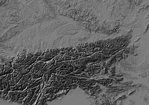
Use GDAL to create hillshade with a simple command. No need to use -s flag to convert units, it already comes in meters. Exaggerate heights a bit with -z flag.

gdaldem hillshade EUD_CP-DEMS_4500025000-AA.tif hillshade.tif -z 3

And here comes the Alps.

To create a color relief you need a ramp of heights with colors. “The Development and Rationale of Cross-blended Hypsometric Tints” by T. Patterson and B. Jenny is a great read on hypsometric tints. They also give advice on what colors to choose in different environments (see the table at the last page of the article). I settled for warm humid color values.

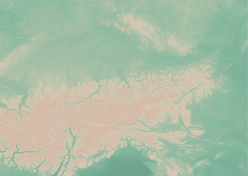
I created a color relief with another GDAL command.

gdaldem color-relief EUD_CP-DEMS_4500025000-AA.tif ramp_humid.txt color_relief.tif

And here comes hypsometric tints.

Add a bit of compression and some overviews to make it smaller and load faster.

gdal_translate -of GTiff -co TILED=YES -co COMPRESS=DEFLATE color_relief.tif color_relief.compress.tif
gdal_translate -of GTiff -co TILED=YES -co COMPRESS=DEFLATE hillshade.tif hillshade.compress.tif
rm color_relief.tif
rm hillshade.tif
mv color_relief.compress.tif color_relief.tif
mv hillshade.compress.tif hillshade.tif
gdaladdo color_relief.tif 2 4 8 16
gdaladdo hillshade.tif 2 4 8 16

Map composition

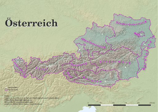
I chose Austria for its excessive amount of freely available datasets. What I didn’t take into consideration was my lack of knowledge when it comes to German (#fail). States come from data.gv.at and was dissolved from smaller administrative units. State capitals were downloaded from naturalearth.com.

I’d like to add some more thematic layers in the future. And translate the map to English.

Few words on INSPIRE Geoportal

INSPIRE Geoportal should be the first place you go to search for European spatial data (at last EU thinks so). I used it to find data for this map and it was a very frustrating experience. It was actually more frustrating than using Austrian open data portal in German. Last news are from May 21, 2015, but the whole site looks and feels like deep 90s or early 2000 at least.

How to Use Queue with Rsync

Having more than 120K 5MB+ images that should be moved to the server is a great oportunity for some automatic bash processing. It might be good idea to use ImageMagick convert tool to make images smaller in a simple for loop. GNU Parallel can significantly increase the performance by running one job per CPU core.

parallel --verbose convert {} -quality 40% {} ::: *.jpg

The parallel modifies several images per second. Uploading these right away seems to be the next step. But how do you tell rsync to check for modified files every now and then? Another for loop mixed with sleep would work, but it just doesn’t feel right.

Luckily, there’s a inotifywait tool capable of watching changes to files and taking actions based on those changes.

inotifywait -e close_write -m --format '%f' . | \
while read file
do
    echo $file
    rsync -OWRD0Pq --ignore-existing $file data@localhost
done

By default, inotifywait stops after receiving a single event, while -m flag runs it indefinitely. -e flag defines an event to watch for, in my case that’s a close_write event. The inotifywait output can be piped to rsync that takes care of syncing local files to remote server.

The last step, as usual, is profit.

Automated Map Creation With QGIS, PostGIS, Python, SVG and ImageMagick

As mentioned in QGIS Tips For Collaborative Mapping we’re in the middle of crop evaluation project at CleverMaps.

With the QGIS workflow up and running, I’ve been focused on different QGIS related task: automatic map generation for land blocks that meet certain conditions. The logic behind identifying such land blocks is as follows:

• if the original area and the measured one differ more than 0.5 % or
• number of declared crops differs from number of crops identified or
• at least one parcel in the land block was given a certain error code

Let’s assume that with several lines of SQL code we can store these mentioned above in a table called land_blocks with geometries being the result of calling ST_Union() over parcels for each land block.

Map composition

Every map should feature following layers:

• land blocks (remember the land_blocks table?) - labeled with ID, yellowish borders, no fill
• land parcels - that’s my source layer - labeled with letters, blue borders, no fill
• other layers
• HR, VHR, NIR imagery, orthophoto - served via WMS

Labels should be visible only for the featured land block (both for the land parcels and the land block itself. The whole map scales dynamically, showing small land blocks zoomed in and the large ones zoomed out.

Every map features additional items:

• dynamic list of subsidies farmer asks for - showing both measured and declared area
• dynamic list of land parcels with their areas and error codes
• scalebar
• map key
• logos

Atlas creation

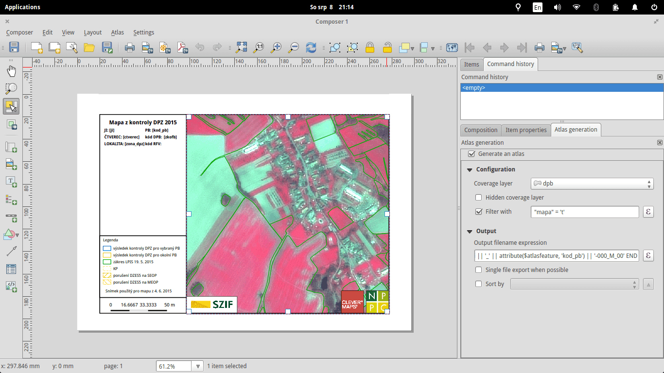
Now with requirements defined, let’s create some maps. It’s incredibly easy to generate a series of maps with QGIS atlas options.

Atlas generation settings

Coverage layer is presumably the only thing you really need - as the name suggests, it covers your area of interest. One map will be created for each feature in this layer, unless you decide to use some filtering - which I did.

Output filenames can be tweaked to your needs, here’s what such a function might look like. If there is a slash in the land block ID (XXXXXXX/Y), the filename is set to USER-ID_XXXXXXX-00Y_M_00, USER-ID_XXXXXXX-000_M_00 otherwise.

CASE WHEN strpos(attribute($atlasfeature, 'kod_pb'), '/') > -1
    THEN
        ji || '_' ||
        substr(
            attribute($atlasfeature, 'kod_pb'), 0,
            strpos(attribute($atlasfeature, 'kod_pb'), '/')+1 -- slash position
        ) || '-' ||
        lpad(
            substr(
                attribute($atlasfeature, 'kod_pb'),
                strpos(attribute($atlasfeature, 'kod_pb'), '/') + 2,
                length(attribute($atlasfeature, 'kod_pb'))
            ),
        3, '0') || '_M_00'
    ELSE
        ji || '_' || attribute($atlasfeature, 'kod_pb') || '-000_M_00'
END

Map scale & variable substitutions

Different land blocks are of different sizes, thus needing different scales to fit in the map. Again, QGIS handles this might-become-a-nightmare-pretty-easily issue with a single click. You can define the scale as:

• margin around feature: percentage of the space displayed around
• predefined scale (best fit): my choice, sometimes it doesn’t display the entire land block though
• fixed scale: sets the scale the same for all the maps

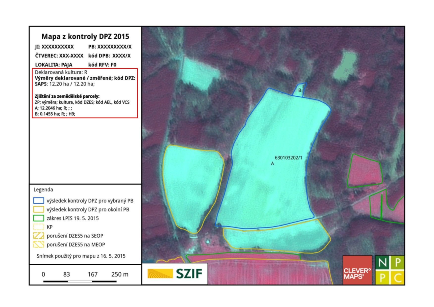
With these settings, I get a map similar to the one below. Notice two interesting things:

• Scale uses decimal places, which I find a huge failure. Has anyone ever seen a map with such scale? The worst is there is no easy way to hide these, or at least I didn’t find one.
• You can see a bunch of [something in the brackets] notations. These will be substituted with actual values during the atlas generation. Showing land block ID with a preceeding label is as easy as [%concat('PB: ', "kod_pb")%] (mind the percentage sign).

Styling the map using atlas features

Atlas features are a great help for map customization. As mentioned earlier, in my case, only one land block label per map should be visible. That can be achieved with a simple label dialog expression:

CASE
    WHEN $id = $atlasfeatureid
    THEN "kod_pb"
END

QGIS keeps reference to each coverage layer feature ID during atlas generation, so you can use it for comparison. The best part is you can use IDs with any layer you need:

CASE
    WHEN attribute($atlasfeature, 'kod_pb') = "kod_pb"
    THEN "kod_zp"
END

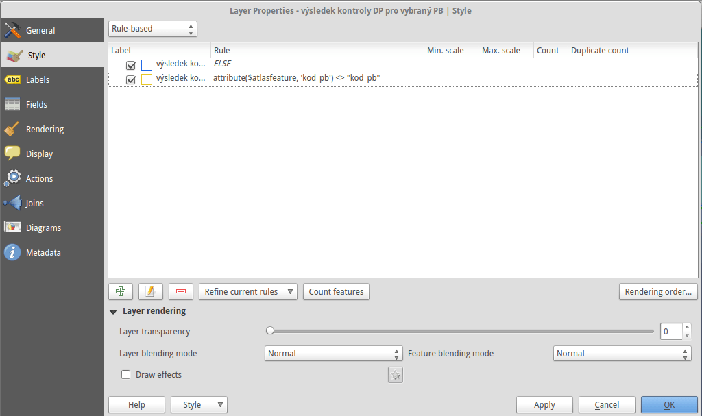
With this simple expression, I get labels only for those land parcels that are part of the mapped land block. Even the layer style can be controlled with atlas feature. Land parcels inside the land block have blue borders, the rest is yellowish, remember? It’s a piece of cake with rule-based styling.

Atlas generation

When you’re set, atlas can be created with a single button. I used SVG as an output format to easily manipulate the map content afterwards. The resulting maps look like the one in the first picture without the text in the red rectangle. A Python script appends this to each map afterwards.

Roughly speaking, generating 300 maps takes an hour or so, I guess that depends on the map complexity and hardware though.

Adding textual content

SVG output is just plain old XML that you can edit by hand or by script. A simple Python script, part of map post-processing, loads SVG from the database and adds it to the left pane of each map.

SELECT
      ji,
      kod_pb,
      concat(
            '<g fill="none" stroke="#000000" stroke-opacity="1" stroke-width="1"
                  stroke-linecap="square" stroke-linejoin="bevel" transform="matrix(1.18081,0,0,1.18081,270.0,550.0)"
                  font-family="Droid Sans" font-size="35" font-style="normal">',
            kultura, vymery, vymery_hodnoty,
            vcs_titul, vcs_brk, vcs_brs, vcs_chmel,
            vcs_zvv, vcs_zv, vcs_ovv, vcs_ov, vcs_cur, vcs_bip,
            lfa, lfa_h1, lfa_h2, lfa_h3,
            lfa_h4, lfa_h5, lfa_oa, lfa_ob, lfa_s,
            natura, aeo_eafrd_text, dv_aeo_eafrd_a1,
            dv_aeo_eafrd_a2o, dv_aeo_eafrd_a2v, dv_aeo_eafrd_b1,
            dv_aeo_eafrd_b2, dv_aeo_eafrd_b3, dv_aeo_eafrd_b4,
            dv_aeo_eafrd_b5, dv_aeo_eafrd_b6, dv_aeo_eafrd_b7,
            dv_aeo_eafrd_b8, dv_aeo_eafrd_b9, dv_aeo_eafrd_c1,
            dv_aeo_eafrd_c3, aeko_text, dv_aeko_a, dv_aeko_b, dv_aeko_c,
            dv_aeko_d1, dv_aeko_d2, dv_aeko_d3, dv_aeko_d4, dv_aeko_d5,
            dv_aeko_d6, dv_aeko_d7, dv_aeko_d8, dv_aeko_d9, dv_aeko_d10,
            dv_aeko_e, dv_aeko_f, ez, dzes_text, rep, obi, seop, meop, pbz, dzes7,
            '</g>'
      ) popis
FROM (...);

Each column from the previous query is a result of SELECT similar to the one below.

SELECT concat('<text fill="#000000" fill-opacity="1" stroke="none">BrK: ', dv_brk, ' ha / ', "MV_BRK", ' ha;', kod_dpz, '</text>') vcs_brk

The transform="matrix(1.18081,0,0,1.18081,270.0,550.0) part puts the text on the right spot. Great finding about SVG is that it places each <text> element on the new line, so you don’t need to deal with calculating the position in your script.

Scale adjustment is done with a dirty lambda function.

content = re.sub(r">(\d{1,3}\.\d{3,5})</text>", lambda m :">    " + str(int(round(float(m.group(1))))) + "</text>", old_map.read())

SVG to JPEG conversion

We deliver maps as JPEG files with 150 DPI on A4 paper format. ImageMagick converts the formats with a simple shell command:

convert -density 150 -resize 1753x1240 input.svg output.jpg

Conclusion

I created pretty efficient semi-automated workflow using several open source technologies that saves me a lot of work. Although QGIS has some minor pet peeves (scale with decimal places, not showing the entire feature, not substituting variables at times), it definitely makes boring map creation quite amusing. The more I work with big data / on big tasks, the more I find Linux a must-have.

The whole process was done with QGIS 2.10, PostGIS 2.1, PostgreSQL 9.3, Python 2.7, ImageMagick 6.7.